08. 모집단과 표본, 모평균의 추정

[엑셀] 실습하기

• 모집단과 표본, 모평균의 추정 (sasa메일로 로그인해야 내용을 볼 수 있습니다.)

[R기초] 실습하기

표본 추출

복원추출(Sampling with replacement)

set.seed(12345)  # 이 명령어는 난수생성기의 초기값을 설정하며, 아무 양수를 넣고 실행 후 아래 명령어를 실행하면, 매번 같은 수가 나옴
sample(x=1:10, size=5, replace=T)  # 1부터 10의 수에서 크기가 5인 표본을 복원추출로 뽑음

[1]  3 10  8 10  8

비복원추출(Sampling without replacement)

set.seed(123)  # 이 명령어를 실행한 후 아래 명령어를 실행하면, 매번 같은 수가 나옴
sample(x=1:10, size=5, replace=F)  # 1부터 10의 수에서 크기가 5인 표본을 비복원추출로 뽑음

[1]  3 10  2  8  6

표본추출예제

• $1$부터 $45$까지 자연수 중 서로 다른 수 $6$개를 추출하시오.

sample(1:45, 6, replace=F) 

[1] 43 37 14 25 26 27

• 등이 나올 확률이 $0.4$인 윷짝 $4$개를 한 번 던지는 모의실험을 하시오.

sample(c(1:0), 4, replace=T, prob=c(0.4, 0.6)) # 등을 1, 배를 0으로 간주함 

[1] 0 0 0 1

• 표준정규분포를 따르는 모집단에서 크기가 $10$인 표본을 임의로 추출하시오.

rnorm(10, 0, 1)

 [1]  1.2240818  0.3598138  0.4007715  0.1106827 -0.5558411  1.7869131
 [7]  0.4978505 -1.9666172  0.7013559 -0.4727914

• 한 개의 주사위를 $1000$번 던질 때, $1$의 눈이 나오는 횟수를 구하는 모의실험을 하시오.

count <- 0
n <- 1
while(n<=1000){
  s <- sample(1:6, 1)
  if(s==1){count <- count+1; n <- n+1}
  else{n <- n+1}
}
count

[1] 170

모집단과 표본

표본평균의 분포

• 히스토그램을 그려 표본수의 증가에 따른 변화를 관찰하기

# 난수발생에 따라 평균값이 xlim=c(0.3, 1.7)을 벗어나거나, 
# 도수가 40보다 많아 ylim=c(0, 40)의 범위를 벗어나는 경우가 있을 수 있다.

par(mfrow=c(2,2))

column_1 <- c()
for (i in 1:100) column_1[i] <- mean(runif(5,0,2)) # 균등분포에서 난수발생하기
hist(column_1, border="white", col="blue", main="mean of 5 samples",
     xlim=c(0.3,1.7), ylim=c(0,40), xlab="Class", ylab="Frequency")

column_2 <- c()
for (i in 1:100) column_2[i] <- mean(runif(10,0,2))
hist(column_2, border="white", col="blue", main="mean of 10 samples",
     xlim=c(0.3,1.7), ylim=c(0,40), xlab="Class", ylab="Frequency")

column_3 <- c()
for (i in 1:100) column_3[i] <- mean(runif(30,0,2))
hist(column_3, border="white", col="blue", main="mean of 30 samples",
     xlim=c(0.3,1.7), ylim=c(0,40), xlab="Class", ylab="Frequency")

column_4 <- c()
for (i in 1:100) column_4[i] <- mean(runif(100,0,2))
hist(column_4, border="white", col="blue", main="mean of 100 samples",
     xlim=c(0.3,1.7), ylim=c(0,40), xlab="Class", ylab="Frequency")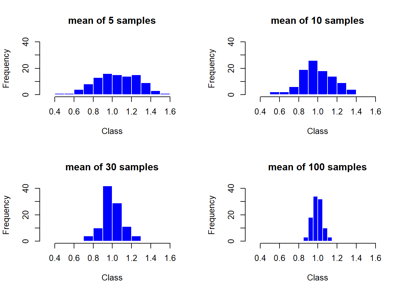

• 표본수의 증가에 따른 기술통계량의 변화를 관찰하기

중심극한정리에 의하면 표본평균 $\overline{X}$의 분포는 이론적으로 평균이 $\mu =\frac{0+2}{2}=1$, 분산이 $\frac{{\sigma }^2}{n}=\frac{(2-0{)}^2}{12}\times \frac{1}{5}=\frac{1}{15}=0.06667$이다. 계산된 요약 통계량을 보면 이론값과 근사적으로 같다는 것을 확인할 수 있다. 최솟값은 점점 커지면서 1로 가고 있고 최댓값은 점점 작아지면서 1로 가고 있기에 대수의 법칙이 작동하고 있음을 알 수 있다.

stat_1 <- c(mean(column_1), var(column_1), median(column_1), 
            min(column_1), max(column_1))
stat_2 <- c(mean(column_2), var(column_2), median(column_2), 
            min(column_2), max(column_2))
stat_3 <- c(mean(column_3), var(column_3), median(column_3), 
            min(column_3), max(column_3))
stat_4 <- c(mean(column_4), var(column_4), median(column_4), 
            min(column_4), max(column_4))

SimStat <- cbind(stat_1, stat_2, stat_3, stat_4) 
rownames(SimStat) <- c("mean", "var", "median", "min", "max")
colnames(SimStat) <- c("n=5", "n=10", "n=30", "n=100") 

SimStat

              n=5       n=10       n=30       n=100
mean   1.04403650 0.99194277 0.99585782 0.993736371
var    0.04754242 0.02959242 0.01132904 0.002992766
median 1.04478925 0.98403686 0.98856144 0.990584588
min    0.43296607 0.50810527 0.71512453 0.877360070
max    1.51308187 1.39665089 1.28565056 1.141150215

t분포

• 표준정규분포 $N(0,1)$을 따르는 확률변수를 $Z$라 하자. 독립적이면서 자유도가 $v$인 카이제곱 분포를 따르는 확률변수를 $V$라고 할 때, $T={\displaystyle \frac{Z}{\sqrt{V/v}}}$의 분포를 자유도가 $v$인 $t$분포라고 한다. 이때 $T\sim t(v)$라고 표시한다.

• $X_1$, $X_2$, $\cdots$, $X_n$ $\sim N(\mu ,{\sigma }^2)$, $\overline{X}\sim N(\mu ,{\displaystyle \frac{{\sigma }^2}{n}})$ 일때, 표준정규분포로 변환이 가능하며, ${\displaystyle \frac{\overline{X}-\mu }{\sigma /\sqrt{n}}}\sim N(0,1)$이다.

• 모분산 ${\sigma }^2$을 모를 때, 표본분산 $S^2={\displaystyle \frac{\sum _{i=1}^n(X_i-\overline{x}{)}^2}{n-1}}$으로 모분산의 추정치로 사용한다.

• 즉, ${\sigma }^2$을 $S^2$으로 추정하면, 자유도가 $n-1$인 $t$분포를 따르게 되며, 이를 표현하면 ${\displaystyle \frac{\overline{X}-\mu }{S/\sqrt{n}}}\sim t(n-1)$이다. ($S$의 자유도가 $n-1$이고, 이것으로부터 $t$분포가 정의되기 때문에 자유도가 $n-1$이다.)

• $t$분포를 따르는 이러한 변환을 스튜던트화(Studentized)라고 하며, $t$분포를 스튜던트 $t$분포라고도 한다.

dt(0, df=30)  # x~t(30)일때, P(x=0)의 값 계산

[1] 0.3956322

dnorm(0, mean=0, sd=1)  #정규분포 Z~N(0,1)의 값과 비교해보면, t분포에서의 값이 약간 작고 따라서 t분포의 양 끝이 조금 두꺼움을 알 수 있다

[1] 0.3989423

pt(0, df=30)  # x~t(30)일때, P(x<0)의 값 계산하면 좌우대칭이라서 0.5임을 알 수 있다

[1] 0.5

pt(1, df=30, lower.tail = T)  # P(x<1)의 값 계산

[1] 0.8373457

pt(1, df=30, lower.tail = F)  # P(x>1)의 값 계산

[1] 0.1626543

pt(1, df=30, lower.tail = T) + pt(1, df=30, lower.tail = F)  # 합이 1임을 확인할 수 있다

[1] 1

qt(0.05, df=30, lower.tail=T)  # 확률이 0.05인 x값

[1] -1.697261

qt(0.025, df=30, lower.tail=T)  # 확률이 0.025인 x값

[1] -2.042272

qt(0.05, df=30, lower.tail=F)  # P(x>x) = 0.05인 x값

[1] 1.697261

qt(0.025, df=30, lower.tail=F)  # P(x>x) = 0.025인 x값

[1] 2.042272

sample = rt(1000, df=30)
hist(sample)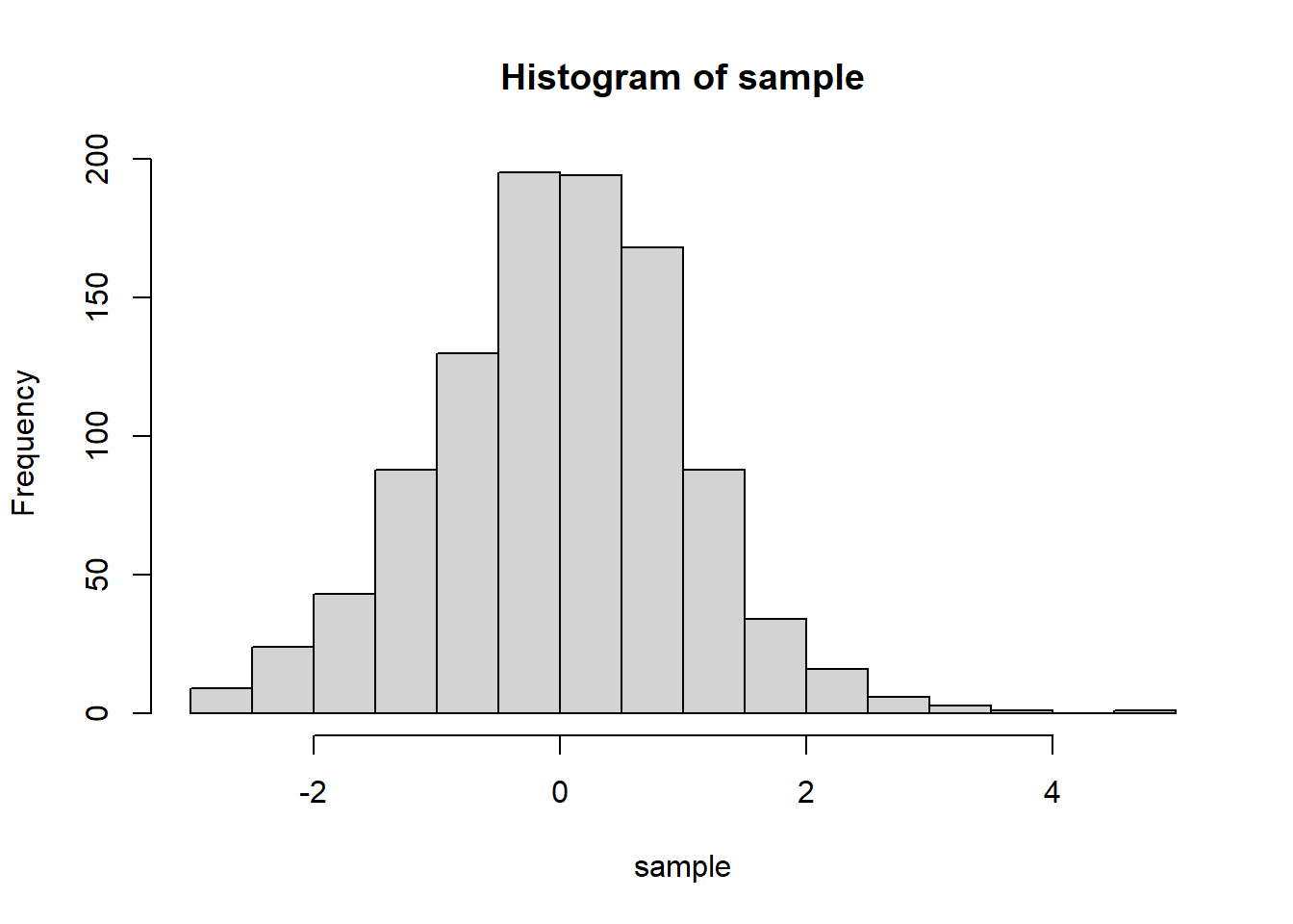

일표본 위치(평균, 중심)에 대한 검증

• 모수적 검정: 데이터가 정규성을 만족하는 경우
• 비모수적 검정: 데이터가 정규성을 만족하지 않는 경우

* 그림 출처: 통계교육원, R을 활용한 통계분석

모평균의 추정

모평균의 구간추정, 신뢰구간

• 다음은 베어링의 평균 직경을 알아보고자 9개의 베어링 표본을 대상으로 조사한 것이다. 3.4, 3.3, 4.2, 4.4, 3.7, 4.5, 4.6, 3.8, 4.1 평균 직경에 대한 95% 신뢰구간을 구하시오.

x <- c(3.4, 3.3, 4.2, 4.4, 3.7, 4.5, 4.6, 3.8, 4.1)

library(TeachingDemos)

Warning: package 'TeachingDemos' was built under R version 4.3.3

z.test(x, sd=0.4, 9)  # 과거로부터 σ=0.4로 알려졌을때 신뢰구간

    One Sample z-test

data:  x
z = -37.5, n = 9.00000, Std. Dev. = 0.40000, Std. Dev. of the sample
mean = 0.13333, p-value < 2.2e-16
alternative hypothesis: true mean is not equal to 9
95 percent confidence interval:
 3.738671 4.261329
sample estimates:
mean of x 
        4 

t.test(x)  # 모표준편차를 모를때 표본표준편차를 이용한 t분포로 구한 신뢰구간

    One Sample t-test

data:  x
t = 25.298, df = 8, p-value = 6.384e-09
alternative hypothesis: true mean is not equal to 0
95 percent confidence interval:
 3.635389 4.364611
sample estimates:
mean of x 
        4 

표본수의 결정

• 앞의 예제에서 오차한계 $d$가 $0.2$라면 표본수 $n$은 얼마가 되어야 하는지 구하시오. ($\alpha =0.05$)

# 오차한계 d=0.2일때때
zstar = qnorm(.975) # σ=0.4로 알려졌을때 n의 개수
sigma = 0.4 
E = 0.2 
zstar^2 * sigma^2/ E^2

[1] 15.36584

zstar = qt(.975, 15) # 모표준편차를 모를때, 자유도를 15로 사용할때의 n의 개수
sigma = 0.4 
E = 0.2 
zstar^2 * sigma^2/ E^2  

[1] 18.17231

zstar = qt(.975, 17) # 모표준편차를 모를때, 자유도를 17로 사용할때의 n의 개수 
sigma = 0.4 
E = 0.2 
zstar^2 * sigma^2/ E^2    

[1] 17.80529

# 따라서 n=18이면 적절하다.