10. 하나의 모집단에 대한 가설검정(평균)

[엑셀] 실습하기

• 하나의 모집단에 대한 가설검정(평균) (sasa메일로 로그인해야 내용을 볼 수 있습니다.)

[R기초] 실습하기

모평균 \(\mu\)에 대한 검정

\(\sigma\)를 아는 경우

• 어떤 이들은 한국 청소년들의 하루 평균 TV 시청 시간이 3시간이라 주장하고, 다른 이들은 공부하느라 시청 시간이 3시간이 안될 것이라 주장하고 있다. 어느 편이 맞는지 알아보기 위하여 단순임의 추출한 100명을 조사한 결과 평균이 2.75시간이었다. TV 시청 시간은 정규분포를 하며 분산은 과거 조사에서 1로 알려져 있다.

# 가설검정을 위한 변수 설정(양측검정)
mu0 <- 3 # 귀무 가설의 평균
xbar <- 2.75 # 표본의 평균
sigma <- 1 # 모집단의 분산 (표준편차)
n <- 100 # 표본의 크기

z <- (xbar - mu0) / (sigma / sqrt(n))  # z-검정 수행
p_value <- 2 * pnorm(-abs(z))  # p-값 계산
z

[1] -2.5

p_value  # 결과 출력

[1] 0.01241933

# p값이 σ=0.05보다 작으므로 귀무가설을 기각하게 되어 
# 청소년들의 하루 평균 TV 시청 시간이 3시간이라고 할 수 없다.

\(\sigma\)를 모르는 경우

• 건강한 성인의 콜레스테롤 수치는 220 이하라고 한다. 콜레스테롤이 높은 사람은 심장마비가 발생할 가능성이 더 높은 것으로 알려져 있다. 이를 확인하기 위해 30명의 심장마비 환자를 조사하여 평균 콜레스테롤이 231이며, 표준편차가 20인 것을 알아냈다. 심장마비 환자들의 평균 콜레스테롤은 정상인의 평균 콜레스테롤보다 높은 수치라고 결론내릴 수 있는가?

t_test <- function(alpha, mu0, xbar, s, n){
    se = s/sqrt(n)
    t = (xbar-mu0)/se
    cr = qt(1-alpha, df=n-1)
    p_value = pt(t, df= n-1, lower.tail=F)
    if(p_value < alpha) result = "Reject H0" else result = "Accept H0"
    
    print(paste("Hypothesis testing for H0: mu = ",mu0,"or Ha: mu > ",mu0))
    print(c(paste("t Statistics is ", round(t,4), 
          "and Critical Region is ", round(cr, 4)), paste("p-value =", round(p_value,4))))
    print(paste(result, "at significance level", alpha))
}

t_test(0.05, 220, 231, 20, 30)  

[1] "Hypothesis testing for H0: mu =  220 or Ha: mu >  220"
[1] "t Statistics is  3.0125 and Critical Region is  1.6991"
[2] "p-value = 0.0027"                                      
[1] "Reject H0 at significance level 0.05"

# p값이 σ=0.05보다 작으므로 귀무가설을 기각하게 되어 
# 심장마비 환자들의 평균 콜레스테롤은 정상의 평균 콜레스테롤보다 높다고 결론을 내린다.

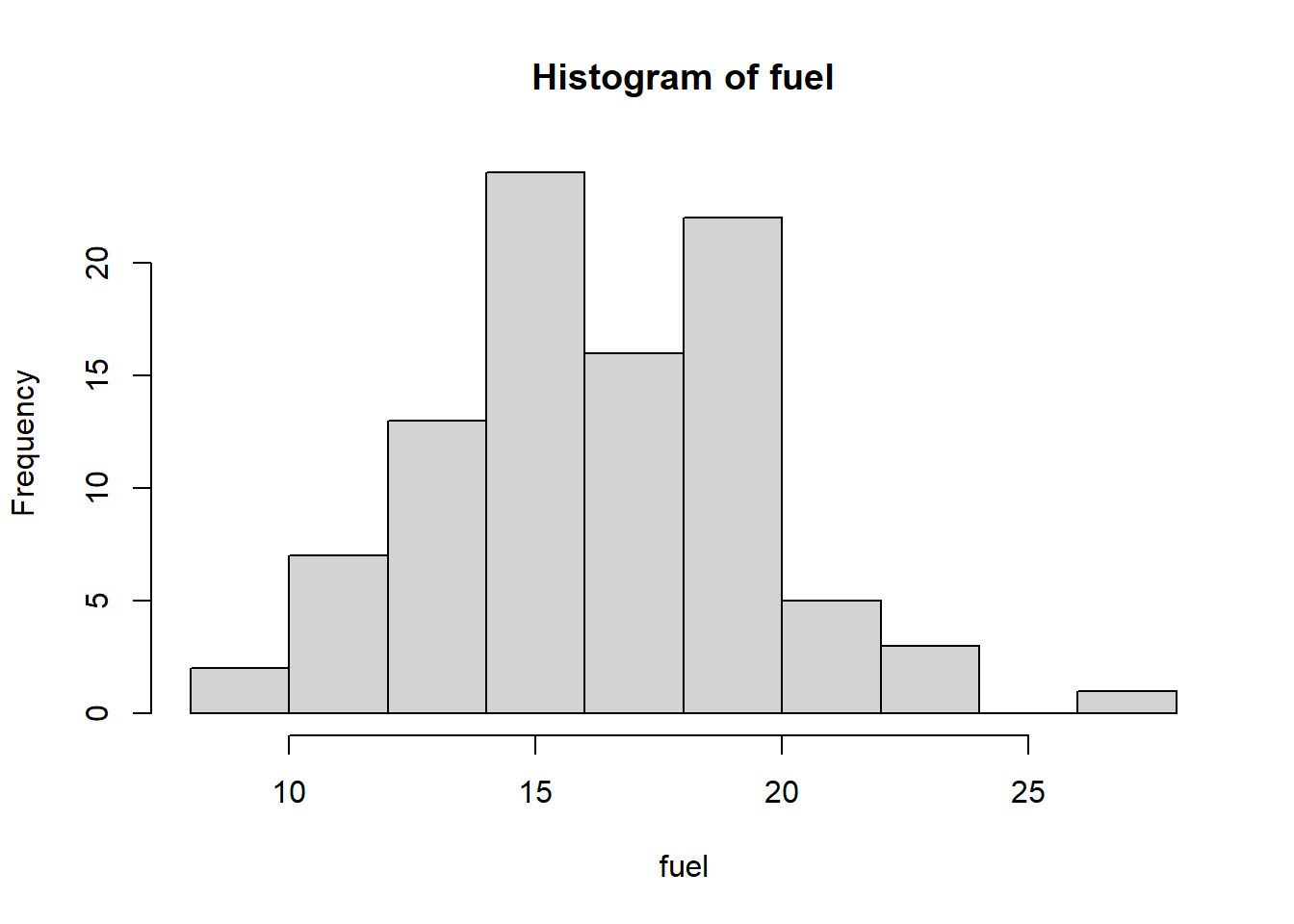
MASS 라이브러리에 있는 Cars93의 연료탱크용량의 모평균 추정하기(t검정)

library(MASS)
fuel = Cars93$Fuel.tank.capacity

## mu of fuel is 16.
# H0: mu = 16
# H1: mu is not 16 (양측검정)

## normality test
hist(fuel)  # 좌우대칭인지 대략적으로 살펴보기

shapiro.test(fuel)  # alpha=0.05 > p ==> H0 reject인데, p=0.287이므로 정규분포를 따름

    Shapiro-Wilk normality test

data:  fuel
W = 0.98341, p-value = 0.287

## 1. hypothesis H0 : mu=16  H1 : mu is not 16
## 2. alpha = 0/05
## 3. test statistic = barX ~ N()
## 4. p
## 5. alpha > p ==> H0 reject

t.test(fuel, mu=16, alternative = 'two.sided')  # p=0.5372 > 0.5이므로 H0를 기각할 수 없고, 즉 연료탱크 용량의 평균은 16이라 할 수 있음

    One Sample t-test

data:  fuel
t = 1.9541, df = 92, p-value = 0.05372
alternative hypothesis: true mean is not equal to 16
95 percent confidence interval:
 15.98914 17.33989
sample estimates:
mean of x 
 16.66452 

t.test(fuel, mu=16, alternative = 'greater')  # p=0.02686 < 0.5이므로 H0를 기각하고, 즉 연료탱크 용량의 평균은 16보다 큼(단측검정이 양측검정보다 귀무가설을 기각하기 쉬움)

    One Sample t-test

data:  fuel
t = 1.9541, df = 92, p-value = 0.02686
alternative hypothesis: true mean is greater than 16
95 percent confidence interval:
 16.09949      Inf
sample estimates:
mean of x 
 16.66452 

t.test(fuel, mu=16, alternative = 'less')  # p=0.9731 > 0.5이므로 H0를 채택한다. 즉 연료탱크 용량의 평균은 16보다 작지 않음

    One Sample t-test

data:  fuel
t = 1.9541, df = 92, p-value = 0.9731
alternative hypothesis: true mean is less than 16
95 percent confidence interval:
     -Inf 17.22955
sample estimates:
mean of x 
 16.66452 

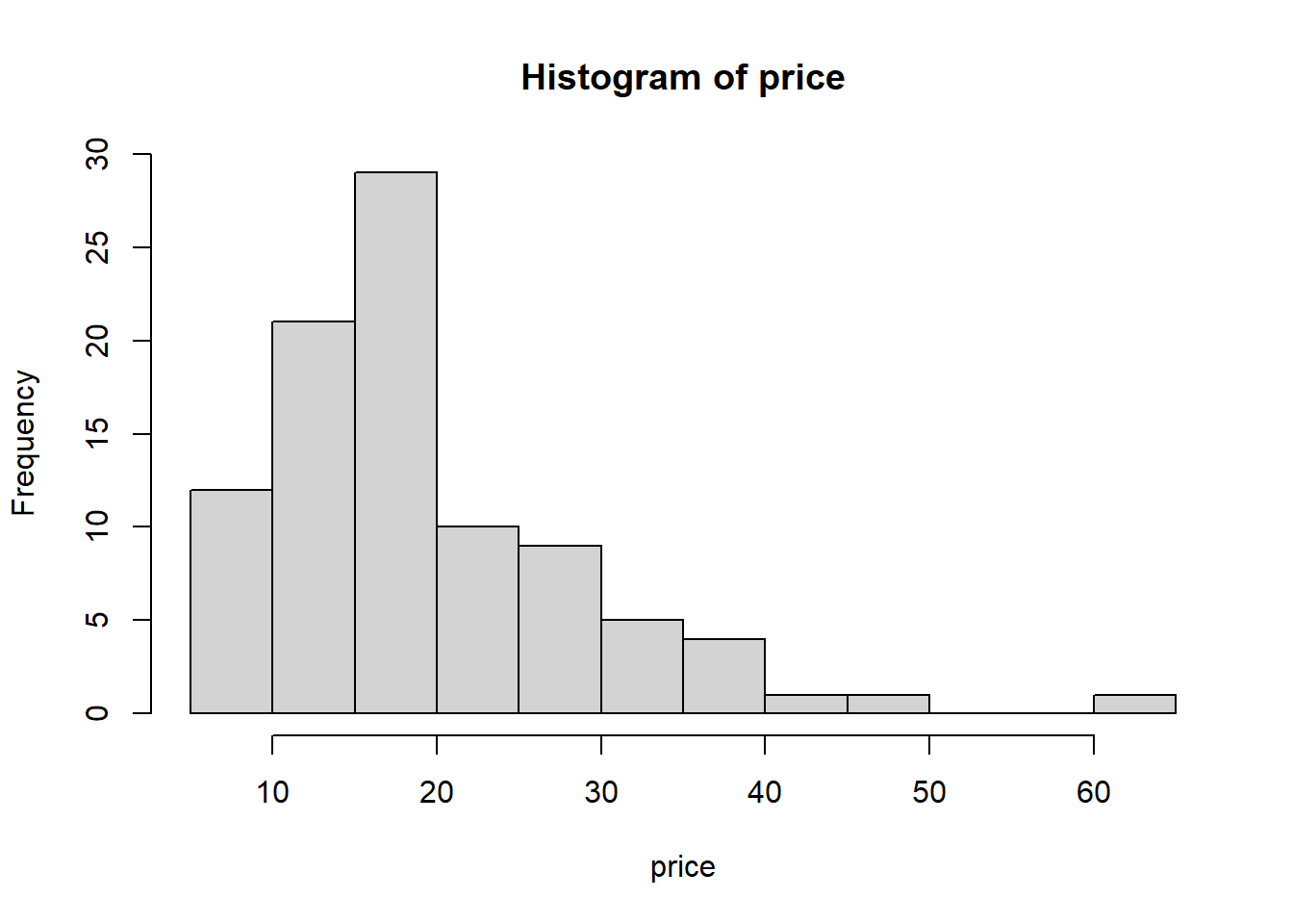
MASS 라이브러리에 있는 Cars93의 가격의 모평균 추정하기(비모수적 방법)

library(MASS)
price = Cars93$Price

## mu of fuel is 16.
# H0: mu = 16
# H1: mu is not 16 (양측검정)

## normality test
hist(price)  # 좌우대칭인지 대략적으로 살펴보기

shapiro.test(price)  # alpha > p ==> H0 reject인데, p=0.0000004235이므로 정규분포를 따른다고 할 수 없음

    Shapiro-Wilk normality test

data:  price
W = 0.88051, p-value = 4.235e-07

## Cars93$Price, nor normal dist~, n>30이면 중심극한정리에 의해 표본평균의 정규성을 활용하여 검정

## n<30(소표본) ==> non-parametric test of one sample(비모수적 방법)
# 1. hypothesis H0 : mu=19  H1 : mu is not 19
# 2. alpha = 0/05

wilcox.test(price, mu=19, alternative = 'two.sided') # 윌콕슨의 부호순위검정, alpha=0.05 > p ==> H0 reject인데, p=0.4701이므로 price의 평균은 19라 할 수 있음

    Wilcoxon signed rank test with continuity correction

data:  price
V = 1953, p-value = 0.4701
alternative hypothesis: true location is not equal to 19

wilcox.test(price, mu=19, alternative = 'greater') # p=0.7662이므로 price의 평균은 19보다 크지 않음

    Wilcoxon signed rank test with continuity correction

data:  price
V = 1953, p-value = 0.7662
alternative hypothesis: true location is greater than 19

wilcox.test(price, mu=19, alternative = 'less') # p=0.235이므로 price의 평균은 19보다 작지 않음

    Wilcoxon signed rank test with continuity correction

data:  price
V = 1953, p-value = 0.235
alternative hypothesis: true location is less than 19

모비율 \(p\)에 대한 검정

• 경기도 어떤 지역에 새로운 지역 신문을 발행하기 위해서는 구독률이 12%를 넘어야 광고주를 안정적으로 확보할 수 있다고 한다. 새로운 지역 신문의 발행을 고심하는 한 신문사에서는 400명의 주민을 대상으로 만약 신문이 발행되면 구독을 할 것인지를 물어서 58명이 구독할 것이라는 답을 얻었다. 새로운 지역 신문의 구독률이 12%를 초과할 것이라고 결론내릴 수 있는가?(유의수준 5% 사용)

prop_test <- function(alpha, p, N, n){
    phat = n/N
    se = sqrt((p*(1-p))/N)
    z = (phat - p) / se
    cr = qnorm(1-alpha)
    p_value = pnorm(z, lower.tail=F)
    if(p_value < alpha) result = "Reject H0" else result = "Accept H0"
    
    print(paste("Hypothesis testing for H0: mu = ",p,"or Ha: mu > ",p))
    print(c(paste("p_hat is ", round(phat,5), "/ Z Statistics is ", round(z,4),
           "and Critical Region is ", round(cr, 4)), paste("p-value =", round(p_value,4))))
    print(paste(result, "at significance level", alpha))
}

prop_test(0.05, 0.12, 400,58)

[1] "Hypothesis testing for H0: mu =  0.12 or Ha: mu >  0.12"
[1] "p_hat is  0.145 / Z Statistics is  1.5386 and Critical Region is  1.6449"
[2] "p-value = 0.0619"                                                        
[1] "Accept H0 at significance level 0.05"

# p값이 유의수준 σ=0.05를 초과하므로 귀무가설을 기각하지 못한다.
# 새로운 지역 신문은 구독률이 12%를 초과할 것이라 결론내릴 수 없다.

• K후보가 소속된 정당에서 K후보 지지율이 0.3인지를 알아보고자 한다. 실제 표본을 1000명을 뽑았을 때, 250명이 K후보를 지지했다고 하자.

# Ho: p=p0,  p=0.3 ?  n= 1000,  X= 250,  approval rating of mr.K =0.3
## alpha = 0.05
## 1) binom.test()
n=1000
x=250
p0=0.3
binom.test(x, n, p=p0, alternative = 'two.sided') # HO reject... p0 is not 0.3 (0.3보다 더 작다고 할 수 있다.)

    Exact binomial test

data:  x and n
number of successes = 250, number of trials = 1000, p-value = 0.0004876
alternative hypothesis: true probability of success is not equal to 0.3
95 percent confidence interval:
 0.2234304 0.2780500
sample estimates:
probability of success 
                  0.25 

## 2) approximate normal distribution
prop.test(x, n, p=p0, alternative = 'two.sided', correct = T) # correct=T(연속성 수정을 함)

    1-sample proportions test with continuity correction

data:  x out of n, null probability p0
X-squared = 11.668, df = 1, p-value = 0.0006359
alternative hypothesis: true p is not equal to 0.3
95 percent confidence interval:
 0.2236728 0.2782761
sample estimates:
   p 
0.25 

prop.test(x, n, p=p0, alternative = 'two.sided', correct = F) # correct=F

    1-sample proportions test without continuity correction

data:  x out of n, null probability p0
X-squared = 11.905, df = 1, p-value = 0.0005599
alternative hypothesis: true p is not equal to 0.3
95 percent confidence interval:
 0.2241531 0.2777603
sample estimates:
   p 
0.25 

• 과거 추석때 귀향률이 20%다. 최근 500명 중 귀향하려는 사람이 79일때 귀향률이 과거보다 줄어들었는지를 알아보고자 한다.

# p0=0.2,  n=500, x=79  H0: p = 0.2  H1 : p<0.2
## 1) binomial distribution
binom.test(79, 500, 0.2, alternative = 'less')

    Exact binomial test

data:  79 and 500
number of successes = 79, number of trials = 500, p-value = 0.009506
alternative hypothesis: true probability of success is less than 0.2
95 percent confidence interval:
 0.0000000 0.1873274
sample estimates:
probability of success 
                 0.158 

## 2) normal distribution with continuity correction
prop.test(79, 500, 0.2, alternative = 'less', correct=T)

    1-sample proportions test with continuity correction

data:  79 out of 500, null probability 0.2
X-squared = 5.2531, df = 1, p-value = 0.01095
alternative hypothesis: true p is less than 0.2
95 percent confidence interval:
 0.0000000 0.1877246
sample estimates:
    p 
0.158 

• ‘Cars93’ 데이터셋에서 변속기 사용 비율이 0.75인지 검정하기

library(MASS)
str(Cars93)

'data.frame':   93 obs. of  27 variables:
 $ Manufacturer      : Factor w/ 32 levels "Acura","Audi",..: 1 1 2 2 3 4 4 4 4 5 ...
 $ Model             : Factor w/ 93 levels "100","190E","240",..: 49 56 9 1 6 24 54 74 73 35 ...
 $ Type              : Factor w/ 6 levels "Compact","Large",..: 4 3 1 3 3 3 2 2 3 2 ...
 $ Min.Price         : num  12.9 29.2 25.9 30.8 23.7 14.2 19.9 22.6 26.3 33 ...
 $ Price             : num  15.9 33.9 29.1 37.7 30 15.7 20.8 23.7 26.3 34.7 ...
 $ Max.Price         : num  18.8 38.7 32.3 44.6 36.2 17.3 21.7 24.9 26.3 36.3 ...
 $ MPG.city          : int  25 18 20 19 22 22 19 16 19 16 ...
 $ MPG.highway       : int  31 25 26 26 30 31 28 25 27 25 ...
 $ AirBags           : Factor w/ 3 levels "Driver & Passenger",..: 3 1 2 1 2 2 2 2 2 2 ...
 $ DriveTrain        : Factor w/ 3 levels "4WD","Front",..: 2 2 2 2 3 2 2 3 2 2 ...
 $ Cylinders         : Factor w/ 6 levels "3","4","5","6",..: 2 4 4 4 2 2 4 4 4 5 ...
 $ EngineSize        : num  1.8 3.2 2.8 2.8 3.5 2.2 3.8 5.7 3.8 4.9 ...
 $ Horsepower        : int  140 200 172 172 208 110 170 180 170 200 ...
 $ RPM               : int  6300 5500 5500 5500 5700 5200 4800 4000 4800 4100 ...
 $ Rev.per.mile      : int  2890 2335 2280 2535 2545 2565 1570 1320 1690 1510 ...
 $ Man.trans.avail   : Factor w/ 2 levels "No","Yes": 2 2 2 2 2 1 1 1 1 1 ...
 $ Fuel.tank.capacity: num  13.2 18 16.9 21.1 21.1 16.4 18 23 18.8 18 ...
 $ Passengers        : int  5 5 5 6 4 6 6 6 5 6 ...
 $ Length            : int  177 195 180 193 186 189 200 216 198 206 ...
 $ Wheelbase         : int  102 115 102 106 109 105 111 116 108 114 ...
 $ Width             : int  68 71 67 70 69 69 74 78 73 73 ...
 $ Turn.circle       : int  37 38 37 37 39 41 42 45 41 43 ...
 $ Rear.seat.room    : num  26.5 30 28 31 27 28 30.5 30.5 26.5 35 ...
 $ Luggage.room      : int  11 15 14 17 13 16 17 21 14 18 ...
 $ Weight            : int  2705 3560 3375 3405 3640 2880 3470 4105 3495 3620 ...
 $ Origin            : Factor w/ 2 levels "USA","non-USA": 2 2 2 2 2 1 1 1 1 1 ...
 $ Make              : Factor w/ 93 levels "Acura Integra",..: 1 2 4 3 5 6 7 9 8 10 ...

## Man.trans.avail 

table(Cars93$Man.trans.avail) #표본수가 크니 prop.test 이용

 No Yes 
 32  61 

## HO : p = 0.75  proportion of Man.trans.avail =0.75
## H1 : p is not 0.75
prop.test(x=61, n=93, p=0.75, alternative = 'two.sided', correct = T)

    1-sample proportions test with continuity correction

data:  61 out of 93, null probability 0.75
X-squared = 3.9032, df = 1, p-value = 0.04819
alternative hypothesis: true p is not equal to 0.75
95 percent confidence interval:
 0.5494157 0.7493692
sample estimates:
       p 
0.655914 

## H1 : p < 0.75
prop.test(x=61, n=93, p=0.75, alternative = 'less', correct = T)

    1-sample proportions test with continuity correction

data:  61 out of 93, null probability 0.75
X-squared = 3.9032, df = 1, p-value = 0.0241
alternative hypothesis: true p is less than 0.75
95 percent confidence interval:
 0.0000000 0.7364348
sample estimates:
       p 
0.655914 

## H1 : p > 0.75
prop.test(x=61, n=93, p=0.75, alternative = 'greater', correct = T)

    1-sample proportions test with continuity correction

data:  61 out of 93, null probability 0.75
X-squared = 3.9032, df = 1, p-value = 0.9759
alternative hypothesis: true p is greater than 0.75
95 percent confidence interval:
 0.5660022 1.0000000
sample estimates:
       p 
0.655914 

두 독립 표본 위치 차이 검정

두 독립 표본 위치 차이 검정이란

통계적 가설검정에서 두 독립 모집단에 대한 평균을 비교하는 검증으로,

• 남녀 간의 성의식 차이
• 농촌과 도시 간의 주거만족도
• 수도권과 비수도권의 삶의 만족도

와 같은 것들을, 보통 \(t\)검정을 통해 두 독립 표본 평균의 차이를 비교한다.

두 독립 모집단의 평균을 비교할 때의 조건

• 두 독립 모집단의 분포는 각각 정규분포여야 함
• 두 독립 모집단이 모두 정규분포이고, 분산이 알려져 있을때 \(\rightarrow\) \(Z\)검정을 통해 평균차이를 검정함
  • \(H_0 : ~ \mu_1 = \mu_2 ~\Rightarrow~ \mu_1 - \mu_2 =0\)
  • 검정통계량: \(X-Y~ \sim ~N \left(\mu_1 - \mu_2 ,~ \dfrac{\sigma^2 _1}{n_1}+ \dfrac{\sigma^2 _2}{n_2} \right)\)
  • 표준화: \(\dfrac{\bar{X}-\bar{Y}-(\mu_1 -\mu_2)}{\sqrt{\dfrac{\sigma^2 _1}{n_1}+ \dfrac{\sigma^2 _2}{n_2}}}~\sim ~N(0,~1)\)
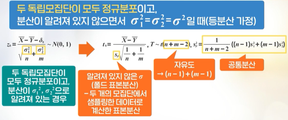
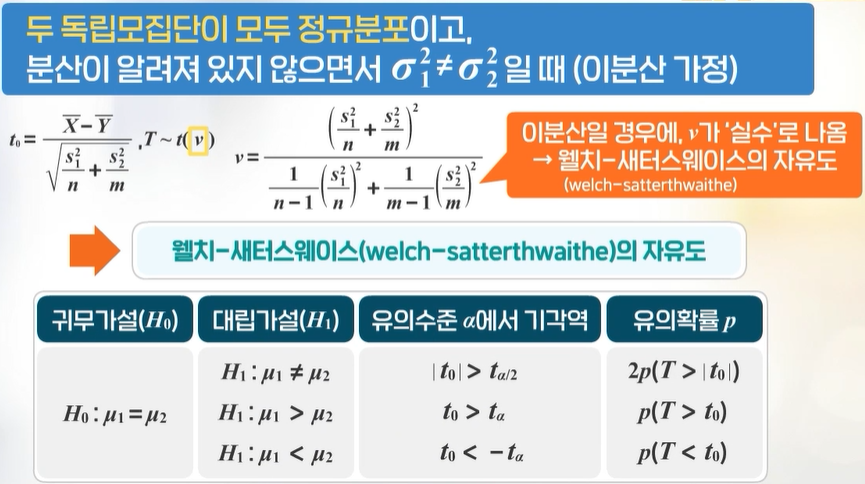
• 두 독립 모집단이 모두 정규분포이고, 분산이 알려져 있지 않을때 \(\rightarrow\) 등분산인지 아닌지 검정 후, \(t\)검정을 통해 평균차이를 검정

  • 등분산을 가정할때:

  • 분산이 같지 않다고 가정할때:

두 독립 모집단의 분산 차이에 대한 등분산성 검정

• 분산이 동일한지 동일하지 않은지에 따라 분산추정량이 달라지기에, 두 집단의 평균을 비교하기 전에 분산의 동일 여부를 검증하며, 이것을 등분산성 검증이라 한다. 아래 귀무가설에서 \(\sigma^2 _1 - \sigma^2 _2 =0\)의 분포 유도는 불가능하기에 귀무가설은 \(\dfrac{\sigma^2 _1 }{\sigma^2 _2}=1\)로 쓸 수 있고, 분산비 \(\dfrac{\sigma^2 _1 }{\sigma^2 _2}=1\)에 대한 추정량은 \(\dfrac{S^2 _1 }{S^2 _2}=1\)이며 \(F\)분포를 따른다.

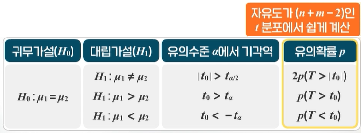
  • 두 독립표본의 모분산에 대한 검정

귀무가설		대립가설
\(H_0 : ~\sigma^2 _1 = \sigma^2 _2\)	VS	\(H_1 : ~\sigma^2 _1 \neq \sigma^2 _2\)(양측검정)
\(H_0 : ~\sigma^2 _1 = \sigma^2 _2\)	VS	\(H_1 : ~\sigma^2 _1 > \sigma^2 _2\) (단측검정)
\(H_0 : ~\sigma^2 _1 = \sigma^2 _2\)	VS	\(H_1 : ~\sigma^2 _1 < \sigma^2 _2\) (단측검정)

• 검정통계량을 통해 분산의 동일 유무 검증은 Levene Test로 한다.

Cars93 데이터셋으로 실습하기

• ‘Cars93’ 데이터셋에서 미국회사 유무(Origin)에 따른 자동차의 가격(Price)에 대한 독립표본 \(t\)검정하기

# two sample t-test
library(MASS)
table(Cars93$Origin)  # 데이터가 30개가 넘으므로 중심극한정리에 의해 정규성을 만족한다고 가정

    USA non-USA 
     48      45 

# equal variance test: leven test,  alpha = 0.05 > p ==> H0 reject
# install.packages("lawstat")  # lawstat 패키지가 없으면 주석을 지우고 설치하기
library(lawstat)  # levene.test()를 하기 위해 패키지 불러오기

Warning: package 'lawstat' was built under R version 4.3.3

levene.test(Cars93$Price, Cars93$Origin, location = 'mean')  # H1 채택, 즉 두 집단의 분산이 다름

    Classical Levene's test based on the absolute deviations from the mean
    ( none not applied because the location is not set to median )

data:  Cars93$Price
Test Statistic = 4.2341, p-value = 0.04248

# two sample t-test
price0 = Cars93$Price[Cars93$Origin == 'USA']
price1 = Cars93$Price[Cars93$Origin != 'USA'] # Cars93$Origin을 치면, non-USA값이지만 왼쪽과 같이 써도 됨

t.test(price0, price1, alternative = 'two.sided', var.equal = FALSE)  # p=0.3428이므로 귀무가설 채택

    Welch Two Sample t-test

data:  price0 and price1
t = -0.95449, df = 77.667, p-value = 0.3428
alternative hypothesis: true difference in means is not equal to 0
95 percent confidence interval:
 -5.974255  2.102311
sample estimates:
mean of x mean of y 
 18.57292  20.50889 

t.test(price0, price1, alternative = 'less', var.equal = FALSE)  # p=0.1714이므로 귀무가설 채택

    Welch Two Sample t-test

data:  price0 and price1
t = -0.95449, df = 77.667, p-value = 0.1714
alternative hypothesis: true difference in means is less than 0
95 percent confidence interval:
     -Inf 1.440539
sample estimates:
mean of x mean of y 
 18.57292  20.50889 

t.test(price0, price1, alternative = 'greater', var.equal = FALSE)  # p=0.8286이므로 귀무가설 채택

    Welch Two Sample t-test

data:  price0 and price1
t = -0.95449, df = 77.667, p-value = 0.8286
alternative hypothesis: true difference in means is greater than 0
95 percent confidence interval:
 -5.312484       Inf
sample estimates:
mean of x mean of y 
 18.57292  20.50889 

• ‘Cars93’ 데이터셋에서 수동변속기의 여부에 따른 자동차의 가격(Price)에 대한 독립표본 \(t\)검정하기

table(Cars93$Man.trans.avail) # 데이터가 30개가 넘으므로 중심극한정리에 의해 정규성을 만족한다고 가정

 No Yes 
 32  61 

# equal variance test
price_0 = Cars93$Price[Cars93$Man.trans.avail == 'Yes']
price_1 = Cars93$Price[Cars93$Man.trans.avail != 'Yes']

levene.test(Cars93$Price, Cars93$Man.trans.avail, location = 'mean')  # p=0.4405이므로 H0 채택, 즉 두 집단은 등분산임

    Classical Levene's test based on the absolute deviations from the mean
    ( none not applied because the location is not set to median )

data:  Cars93$Price
Test Statistic = 0.60016, p-value = 0.4405

t.test(price_0, price_1, alternative = 'two.sided', var.equal = TRUE)  # p=0.001403이므로 H1 채택, 즉 수동변속기 유무에 따른 두 집단의 가격이 다르다 할 수 있음 

    Two Sample t-test

data:  price_0 and price_1
t = -3.2952, df = 91, p-value = 0.001403
alternative hypothesis: true difference in means is not equal to 0
95 percent confidence interval:
 -10.583164  -2.622676
sample estimates:
mean of x mean of y 
 17.23770  23.84062 

t.test(price_0, price_1, alternative = 'less', var.equal = TRUE)  # p=0.0007013으로 양측검정때보다 더 작아짐

    Two Sample t-test

data:  price_0 and price_1
t = -3.2952, df = 91, p-value = 0.0007013
alternative hypothesis: true difference in means is less than 0
95 percent confidence interval:
      -Inf -3.273112
sample estimates:
mean of x mean of y 
 17.23770  23.84062 

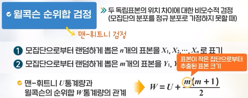
두 독립 모집단의 정규성을 보장하지 못할 때, 평균 차이에 대한 비모수적 검정

윌콕슨 순위합 검정이란

예제로 실습하기

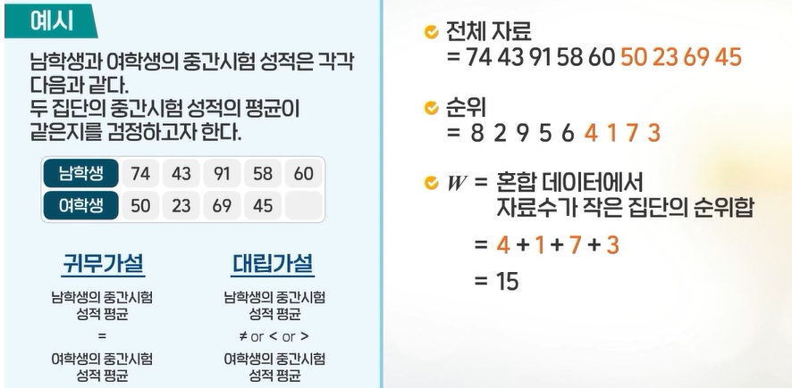
• 남학생과 여학생의 중간시험 성적이 각각 다음과 같을때, 두 집단의 중간시험 성적의 평균이 같은지를 검정하고자 한다. 남학생: 74, 43, 91, 58, 60, 여학생: 50, 23, 69, 45

# 13 wilcoxon rank sum test for two sample 

male = c(74, 43, 91, 58, 60)
female = c(50, 23, 69, 45)
shapiro.test(male) # normality test

    Shapiro-Wilk normality test

data:  male
W = 0.97284, p-value = 0.8932

shapiro.test(female) # 정규분포를 따른다고 p값이 나오지만 표본수가 적어서 정규분포를 따른다는 가정을 못하고, 윌콕슨 검정하기

    Shapiro-Wilk normality test

data:  female
W = 0.98134, p-value = 0.9098

data = c(male, female) # 데이터 합치기
rank_data = rank(data) # 데이터의 순위를 매기기
rank_data

[1] 8 2 9 5 6 4 1 7 3

female_seq = seq(length(male)+1, length(data)) # 여성 자료의 위치
female_seq

[1] 6 7 8 9

female_rank = rank_data[female_seq]
female_rank

[1] 4 1 7 3

W = sum(female_rank)  # 더 적은 집단의 합을 W로 함
W  # 수작업으로 W구하기

[1] 15

wilcox.test(male, female, alternative = 'two.sided') # 바로 W를 구하고, p값 구함, (alpha = 0.05 > p ==> H0 reject) H0를 채택함, 즉 여학생과 남학생의 성적 평균의 차이가 없음

    Wilcoxon rank sum exact test

data:  male and female
W = 15, p-value = 0.2857
alternative hypothesis: true location shift is not equal to 0

Cars93 데이터셋으로 실습하기

• ‘Cars93’ 데이터셋에서 미국회사 유무에 따른 자동차의 가격(Price)에 대한 독립표본 윌콕슨 순위합 검정

library(MASS)
table(Cars93$Origin)

    USA non-USA 
     48      45 

# wilcoxon rank sum test , alpha = 0.05 > p ==> Ho rejcet

price_0 = Cars93$Price[Cars93$Origin == 'USA']
price_1 = Cars93$Price[Cars93$Origin != 'USA']
wilcox.test(price_0, price_1, alternative = 'two.sided') # p값 ==> H0 채택, 즉 가격 차이가 없음

Warning in wilcox.test.default(price_0, price_1, alternative = "two.sided"):
cannot compute exact p-value with ties

    Wilcoxon rank sum test with continuity correction

data:  price_0 and price_1
W = 1024.5, p-value = 0.6724
alternative hypothesis: true location shift is not equal to 0

wilcox.test(price_0, price_1, alternative = 'less') # p값 ==> H0 채택

Warning in wilcox.test.default(price_0, price_1, alternative = "less"): cannot
compute exact p-value with ties

    Wilcoxon rank sum test with continuity correction

data:  price_0 and price_1
W = 1024.5, p-value = 0.3362
alternative hypothesis: true location shift is less than 0

wilcox.test(price_0, price_1, alternative = 'greater') # p값 ==> H0 채택

Warning in wilcox.test.default(price_0, price_1, alternative = "greater"):
cannot compute exact p-value with ties

    Wilcoxon rank sum test with continuity correction

data:  price_0 and price_1
W = 1024.5, p-value = 0.6666
alternative hypothesis: true location shift is greater than 0

• ‘Cars93’ 데이터셋에서 수동변속기 유무에 따른 자동차의 가격(Price)에 대한 독립표본 윌콕슨 순위합 검정

price0 = Cars93$Price[Cars93$Man.trans.avail == 'Yes']
price1 = Cars93$Price[Cars93$Man.trans.avail != 'Yes']

wilcox.test(price0, price1, alternative = 'two.sided') # p값 ==> H0 기각, 즉 가격 차이가 있음

    Wilcoxon rank sum test with continuity correction

data:  price0 and price1
W = 530.5, p-value = 0.0003196
alternative hypothesis: true location shift is not equal to 0

wilcox.test(price0, price1, alternative = 'less') # p값 ==> H0 기각

    Wilcoxon rank sum test with continuity correction

data:  price0 and price1
W = 530.5, p-value = 0.0001598
alternative hypothesis: true location shift is less than 0

wilcox.test(price0, price1, alternative = 'greater') # 'less'가 가장 적당하다는 것을 알 수 있음

    Wilcoxon rank sum test with continuity correction

data:  price0 and price1
W = 530.5, p-value = 0.9998
alternative hypothesis: true location shift is greater than 0

대응표본 평균 차이 검정

하나의 자료에 두 개의 대응되는 변수가 있을때, 두 변수의 평균의 차이가 있는지 검정하는 것

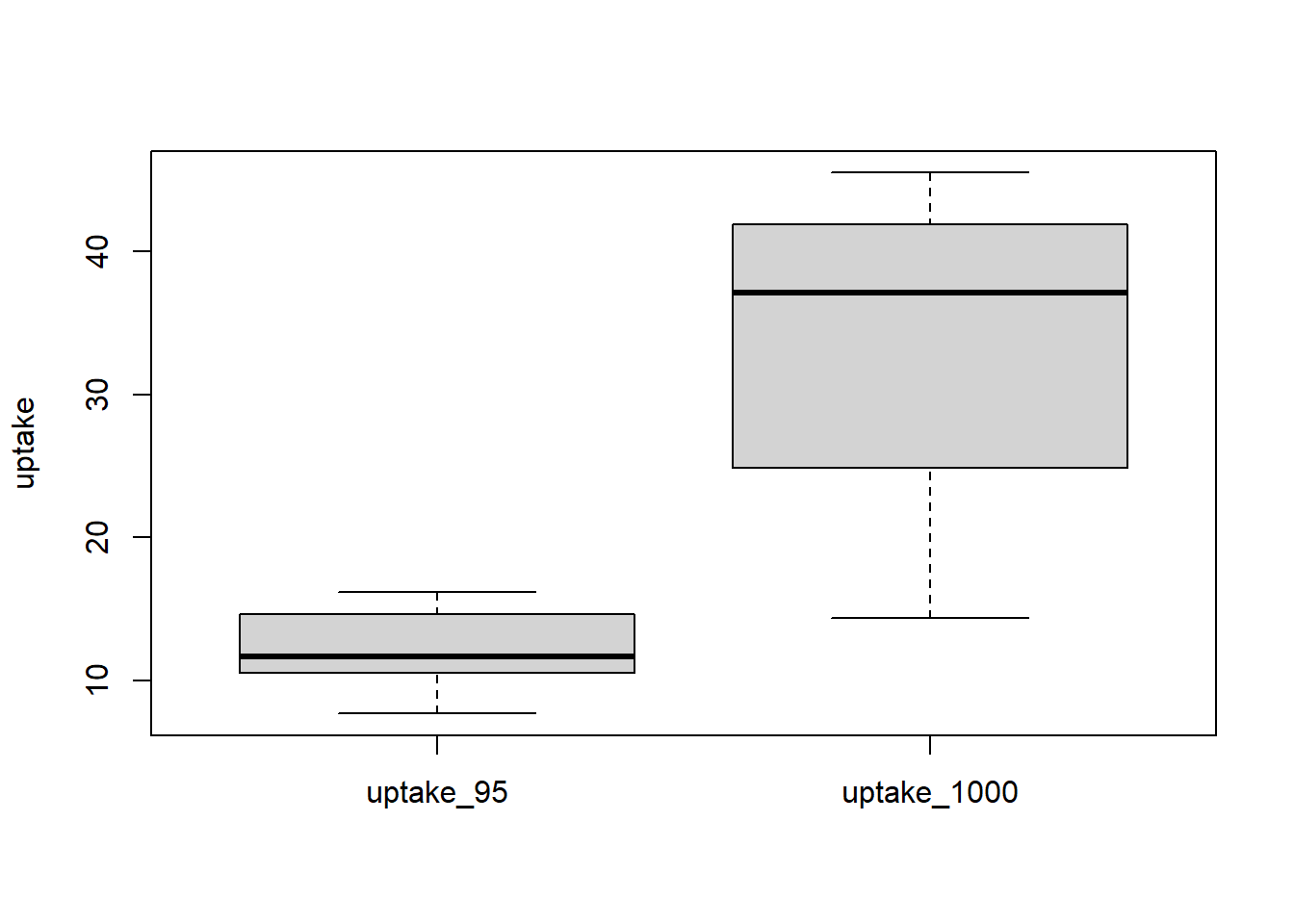
주변 이산화탄소 농도에 따른 나무의 이산화탄소 흡수율 차이 검정

데이터의 모양은 다음과 같다.

## paired t-test
## uptake of CO2
str(CO2)  # 데이터 구조 확인

Classes 'nfnGroupedData', 'nfGroupedData', 'groupedData' and 'data.frame':  84 obs. of  5 variables:
 $ Plant    : Ord.factor w/ 12 levels "Qn1"<"Qn2"<"Qn3"<..: 1 1 1 1 1 1 1 2 2 2 ...
 $ Type     : Factor w/ 2 levels "Quebec","Mississippi": 1 1 1 1 1 1 1 1 1 1 ...
 $ Treatment: Factor w/ 2 levels "nonchilled","chilled": 1 1 1 1 1 1 1 1 1 1 ...
 $ conc     : num  95 175 250 350 500 675 1000 95 175 250 ...
 $ uptake   : num  16 30.4 34.8 37.2 35.3 39.2 39.7 13.6 27.3 37.1 ...
 - attr(*, "formula")=Class 'formula'  language uptake ~ conc | Plant
  .. ..- attr(*, ".Environment")=<environment: R_EmptyEnv> 
 - attr(*, "outer")=Class 'formula'  language ~Treatment * Type
  .. ..- attr(*, ".Environment")=<environment: R_EmptyEnv> 
 - attr(*, "labels")=List of 2
  ..$ x: chr "Ambient carbon dioxide concentration"
  ..$ y: chr "CO2 uptake rate"
 - attr(*, "units")=List of 2
  ..$ x: chr "(uL/L)"
  ..$ y: chr "(umol/m^2 s)"

uptake_95   = CO2[CO2$conc == 95, ]$uptake  # 주변 이산화탄소의 농도가 95일때 흡수율
uptake_1000 = CO2[CO2$conc == 1000, ]$uptake  # 주변 이산화탄소의 농도가 1000일때 흡수율
uptake_95

 [1] 16.0 13.6 16.2 14.2  9.3 15.1 10.6 12.0 11.3 10.5  7.7 10.6

uptake_1000

 [1] 39.7 44.3 45.5 38.7 42.4 41.4 35.5 31.5 27.8 21.9 14.4 19.9

boxplot(data.frame(uptake_95, uptake_1000),  # 상자 그림을 그려서 데이터 분포 확인
        ylab='uptake')

# paired t-test : HO : mu_d = 0, mu_d is no 0
## 1. compare two variance 
var.test(uptake_95, uptake_1000) # 한 모집단 내 두 변수의 등분산성 검정, H0: equal variance ==> not equal variance

    F test to compare two variances

data:  uptake_95 and uptake_1000
F = 0.069007, num df = 11, denom df = 11, p-value = 0.0001066
alternative hypothesis: true ratio of variances is not equal to 1
95 percent confidence interval:
 0.01986555 0.23970934
sample estimates:
ratio of variances 
        0.06900694 

## 2. t-test, 두 대응표본의 이산화탄소 흡수율(uptake)에 대해 대응표본 t검정
t.test(uptake_95, uptake_1000, paired = TRUE, # paired 파라미터를 TRUE로 설정하면 대응표본 t검정 실시
       var.equal = FALSE, alternative = 'two.sided') ## reject H0, H1 채택, 주변이산화탄소 농도에 따른 이산화탄소 흡수율에 차이가 있다 할 수 있음

    Paired t-test

data:  uptake_95 and uptake_1000
t = -8.5197, df = 11, p-value = 3.573e-06
alternative hypothesis: true mean difference is not equal to 0
95 percent confidence interval:
 -26.83414 -15.81586
sample estimates:
mean difference 
        -21.325 

중간고사와 기말고사의 평균 비교(5명이니 소표본임)

# 수치형 변수이고, 표본이 작을 때 두 변수의 평균을 비교하는 비모수적 방법: 윌콕슨 부호 순위 검정
## non-parametric paired test : wilcoxon signed rank test

midterm = c(80, 70, 62, 92, 87)
final =   c(82, 72, 60, 91, 75)

wilcox.test(midterm, final, alternative = 'two.sided',
            paired = TRUE)  # H0 채택, 즉 차이가 없다.

Warning in wilcox.test.default(midterm, final, alternative = "two.sided", :
cannot compute exact p-value with ties

    Wilcoxon signed rank test with continuity correction

data:  midterm and final
V = 9, p-value = 0.7835
alternative hypothesis: true location shift is not equal to 0

## tie(동점)가 있는 경우 ==> wilcoxon test ==> wilcox.exact() function
# install.packages('exactRankTests')  # 라이브러리가 없으면 주석 지우고 설치하기
library(exactRankTests)

Warning: package 'exactRankTests' was built under R version 4.3.3

 Package 'exactRankTests' is no longer under development.
 Please consider using package 'coin' instead.

wilcox.exact(midterm, final, alternative = 'two.sided',
             paired = TRUE)  # H0 채택, 즉 차이가 없다.

    Exact Wilcoxon signed rank test

data:  midterm and final
V = 9, p-value = 0.8125
alternative hypothesis: true mu is not equal to 0

두 모집단에 대한 비율 차이 검정 예제

여러 독립 모집단의 모비율 차이에 대한 검정도 두 독립모집단의 모비율 차이와 동일하게 검토할 수 있다. 독감예방주사여부에 따른 감기증세 비율 예제를 통해 이항분포를 활용하여 검정하는 방법과 정규근사를 활용하여 검정하는 두 가지 방법을 배워보자. 그리고 Cars93 데이터셋에서 prop.test()으로 검정하는 것도 배워보자.

• 독감예방백신주사를 맞은 집단과 맞지 않은 집단에서의 감기증세를 보이는 비율 차이 검정

# significant test for two-sample proportion 

# 1. binomial distribution
## binom.test(x, n, p0, alternative='two.sided'): 하나의 모비율에 대한 검정
## binom.test(x-vector, n-vector, ~): 두 모비율의 차이에 대한 검정

## H0: p1 = p2   p1: shot   p2: not-shot
## H1: p1 is not p2
# shot    : n1 = 201    number of catch cold x1=11  
# not-shot: n2 = 200    number of catch cold x2=33
# alpha = 0.05

n1=201  #독감예방접종을 한 사람
n2=200  #독감예방접종을 안한 사람
x1=11  #n1에서 감기증세 있는 사람 수
x2=33  #n2에서 감기증세 있는 사람 수

n = c(n1, n2)
x = c(x1, x2)
binom.test(x, n, alternative = 'two.sided') #검정결과 두 집단에서 감기증세를 보이는 사람의 비율은 같지 않음

    Exact binomial test

data:  x
number of successes = 11, number of trials = 44, p-value = 0.00126
alternative hypothesis: true probability of success is not equal to 0.5
95 percent confidence interval:
 0.1319274 0.4033804
sample estimates:
probability of success 
                  0.25 

## H1: p1 < p2
binom.test(x, n, alternative = 'less') #검정결과 독감주사를 맞은 집단이 감기 걸릴 확률이 더 낮음

    Exact binomial test

data:  x
number of successes = 11, number of trials = 44, p-value = 0.00063
alternative hypothesis: true probability of success is less than 0.5
95 percent confidence interval:
 0.0000000 0.3797055
sample estimates:
probability of success 
                  0.25 

## normal distribution(n이 크므로 정규분포의 근사를 활용하여 검정)
prop.test(x, n, alternative = 'two.sided', correct = T) #검정결과 귀무가설 기각으로 두 모비율이 차이가 있음.(함수 내부적으로 카이제곱검정 사용)

    2-sample test for equality of proportions with continuity correction

data:  x out of n
X-squared = 11.376, df = 1, p-value = 0.000744
alternative hypothesis: two.sided
95 percent confidence interval:
 -0.17555184 -0.04499543
sample estimates:
    prop 1     prop 2 
0.05472637 0.16500000 

prop.test(x, n, alternative = 'less', correct = T) #단측검정을 하면 p값이 더 작아지고, 더 잘 기각하게 됨. 즉 독감예방주사를 맞은 집단이 모비율이 더 작음

    2-sample test for equality of proportions with continuity correction

data:  x out of n
X-squared = 11.376, df = 1, p-value = 0.000372
alternative hypothesis: less
95 percent confidence interval:
 -1.00000000 -0.05468857
sample estimates:
    prop 1     prop 2 
0.05472637 0.16500000 

• Cars93 데이터셋에서 미국회사 여부(Origin)에 따른 두 집단의 수동변속기 사용 가능 비율에 대한 모비율 검정

library(MASS)
## Origin: USA, non-USA
## Man.trans.avail: 수동변속기 사용 여부

table(Cars93[ , c('Man.trans.avail', 'Origin')])

               Origin
Man.trans.avail USA non-USA
            No   26       6
            Yes  22      39

## H0: p1 of USA = p2 of non-USA  Yes prop of Man.trans.avail 
## H1: p1 is not p2

n = c(48, 45) #미국회사 유무에 따른 차량수
x = c(22, 39) #수동변속기 사용 가능한 차량수
prop.test(x, n, alternative = 'two.sided') #모비율을 검정하는 내장함수, 검정결과 귀무가설 기각, 즉 비율이 다름

    2-sample test for equality of proportions with continuity correction

data:  x out of n
X-squared = 15.397, df = 1, p-value = 8.712e-05
alternative hypothesis: two.sided
95 percent confidence interval:
 -0.6022941 -0.2143725
sample estimates:
   prop 1    prop 2 
0.4583333 0.8666667 

prop.test(x, n, alternative = 'less') #정보를 더 알면 단측검정이 유리함

    2-sample test for equality of proportions with continuity correction

data:  x out of n
X-squared = 15.397, df = 1, p-value = 4.356e-05
alternative hypothesis: less
95 percent confidence interval:
 -1.0000000 -0.2420952
sample estimates:
   prop 1    prop 2 
0.4583333 0.8666667 

prop.test(x, n, alternative = 'greater') #이 경우는 할 필요가 없다는 것을 알 수 있음

    2-sample test for equality of proportions with continuity correction

data:  x out of n
X-squared = 15.397, df = 1, p-value = 1
alternative hypothesis: greater
95 percent confidence interval:
 -0.5745715  1.0000000
sample estimates:
   prop 1    prop 2 
0.4583333 0.8666667