두개의 변량에 대해 서로 상관되는 인자항목들이 어떤 관련성이 있고, 그 관련성이 어느 정도인지를 수치적으로 분석하는 것을 상관분석(correlation analysis)이라 하며, 실제 관측된 값과 모형의 결과를 서로 비교할 때 상관분석을 통하여 모형의 적합성 정도를 표현하기도 한다. 상관계수는 pearson, spearman, kendall의 3가지 상관계수가 있으며, \(-1 \sim 1\)의 값을 가지는데 두 변수가 음의 상관성을 가질수록 \(-1\), 양의 상관성을 가질수록 \(1\), 상관성을 가지지 않을수록 \(0\)과 가깝게 나타난다.
R 내장함수 corr()로 pearson, spearman, kendall 상관계수를 구할 수 있다. corr()의 파라미터 method에 아무것도 지정하지 않으면, pearman, ’spearman’으로 지정하면 spearman, ’kendall’로 지정하면 kendall 상관계수가 출력된다.
상관분석: 모수적 상관분석
Pearson 상관분석
두 변수가 모두 수치형 변수인 경우 일반적으로 pearson의 상관계수를 계산한다.
pearson 상관계수는 대표본이거나 각 변수의 모집단분포가 정규분포인 경우, \((x_i ,\ y_i)\)와 같은 순서쌍으로 주어진다. 모집단의 상관계수는 모수로서 일반적으로 알려져 있지 않다.
모집단으로부터 랜덤하게 \(n\)개를 표본으로 뽑은 경우, \((x_1 ,\ y_1)\), \(\cdots\) , \((x_n ,\ y_n)\)의 표본의 순서쌍에서 표본상관계수를 계산할 수 있다.(\(S_{x}\): \(X\)의 표준편차, \(S_{y}\): \(Y\)의 표준편차, \(S_{xy}\): \(X\)와 \(Y\)의 공분산)
\[
r=\dfrac{S_{xy}}{S_{x}S_{y}}
\]
표본상관계수 \(r\)을 가지고 모상관계수 \(\rho\)에 대한 가설검정을 할 수 있다.
귀무가설\(~ ~H_0 : \rho=0\) (모집단에서는 두 변수 간에 상관관계가 없다.)
대립가설
\(~ ~ ~ ~ ~ ~ ~H_1 : \rho\neq0\) (모집단에서는 두 변수 간에 상관관계가 있다.)[양측검정]
\(~ ~ ~ ~ ~ ~ ~H_1 : \rho>0\) (모집단에서는 두 변수 간에 양의 상관관계가 있다.)[단측검정]
\(~ ~ ~ ~ ~ ~ ~H_1 : \rho<0\) (모집단에서는 두 변수 간에 음의 상관관계가 있다.)[단측검정]
자유도가 \(n-2\)인 \(t\)분포를 따르므로 표본상관계수에 대해서 \(t\)검정을 한다.
\(t\)분포를 이용하여 유의확률 \(p\)를 계산했을 대 유의수준 \(\alpha\)보다 작으면 귀무가설을 기각한다.
상관분석: 비모수적 상관분석
Spearman의 순위상관계수
비모수적 상관계수이다.
소표본이며 변수의 분포가 정규분포라고 할 수 없을 때, 각 변수의 순위를 가지고 순위에 대한 pearson 상관계수를 구하는 공식으로 계산한다.
유의성 검정은 pearson의 상관과는 달리 비모수적 검정에 의해 실시한다.
Kendall’s Tau(켄달의 순위상관계수)
spearman 순위상관계수처럼 두 변수 사이의 연관성을 나타내는 비모수적 방법이다.
\((x_1 ,\ y_1)\), \(\cdots\) , \((x_n ,\ y_n)\)의 순서쌍에서 모든 \(i<j\)에 대해 \(P=(x_i - x_j)(y_i - y_j)>0\)인 쌍의 개수, \(Q=(x_i - x_j)(y_i - y_j)<0\)인 쌍의 개수일 때, 켄달의 타우는 다음 식과 같다.
\[
Kendall's \ \tau =\dfrac{P-Q}{P+Q}
\]
[R기초] 실습하기
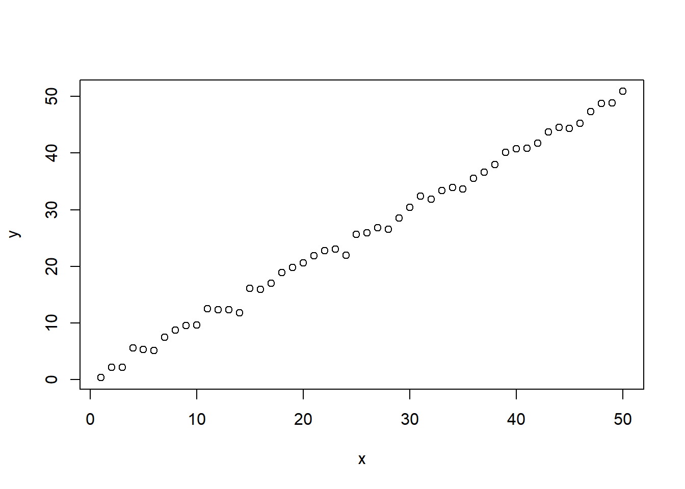
선형적 자료에 대한 상관분석
## correlation analaysis## 1. linear data x=c(1:50) ; x
###1) pearson correlation coefficientcor(x, y) #상관계수 구하기
[1] 0.9983757
## significant test(유의성 검정)cor.test(x, y) # HO: x and y are independent, 검정결과 귀무가설 기각
    Pearson's product-moment correlation

data:  x and y
t = 121.41, df = 48, p-value < 2.2e-16
alternative hypothesis: true correlation is not equal to 0
95 percent confidence interval:
 0.9971245 0.9990827
sample estimates:
      cor
0.9983757
###2) spearman correlation coefficientcor(x, y, method ='spearman') #상관계수 구하기
[1] 0.9977911
cor.test(x, y, method ='spearman') #유의성 검정
    Spearman's rank correlation rho

data:  x and y
S = 46, p-value < 2.2e-16
alternative hypothesis: true rho is not equal to 0
sample estimates:
      rho
0.9977911
###3) kendall correlation coefficientcor(x, y, method ='kendall') #상관계수 구하기
[1] 0.9722449
cor.test(x,y, method ='kendall') #유의성 검정
    Kendall's rank correlation tau

data:  x and y
z = 9.9625, p-value < 2.2e-16
alternative hypothesis: true tau is not equal to 0
sample estimates:
      tau
0.9722449
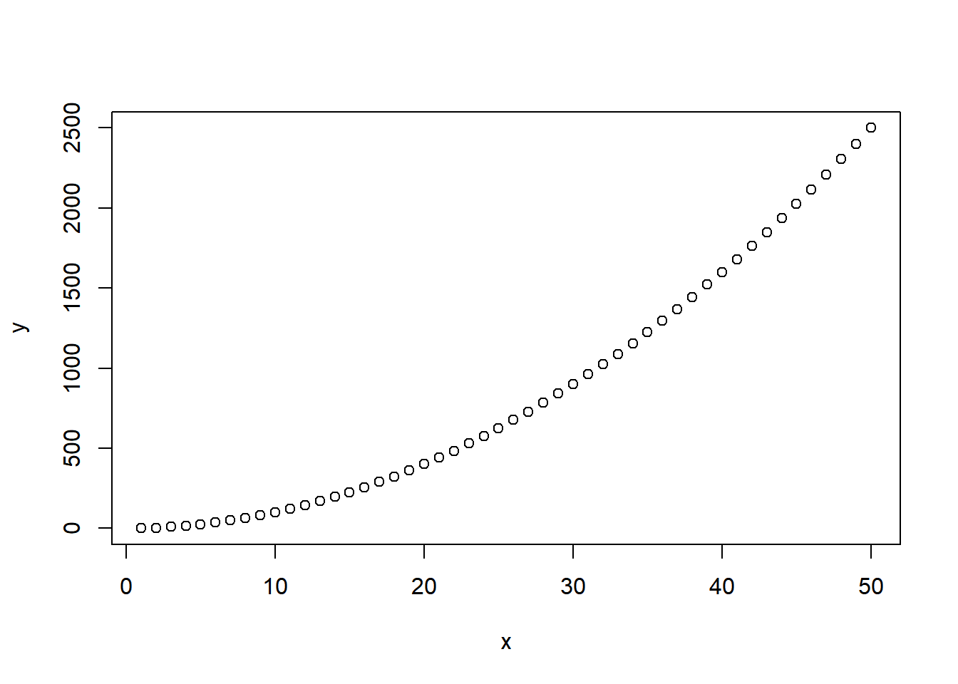
    Pearson's product-moment correlation

data:  x and y
t = 27.391, df = 48, p-value < 2.2e-16
alternative hypothesis: true correlation is not equal to 0
95 percent confidence interval:
 0.9465474 0.9826497
sample estimates:
      cor
0.9694696
cor.test(x,y, method='spearman')
    Spearman's rank correlation rho

data:  x and y
S = 0, p-value < 2.2e-16
alternative hypothesis: true rho is not equal to 0
sample estimates:
rho
  1
cor.test(x,y, method='kendall')
    Kendall's rank correlation tau

data:  x and y
z = 10.247, p-value < 2.2e-16
alternative hypothesis: true tau is not equal to 0
sample estimates:
tau
  1
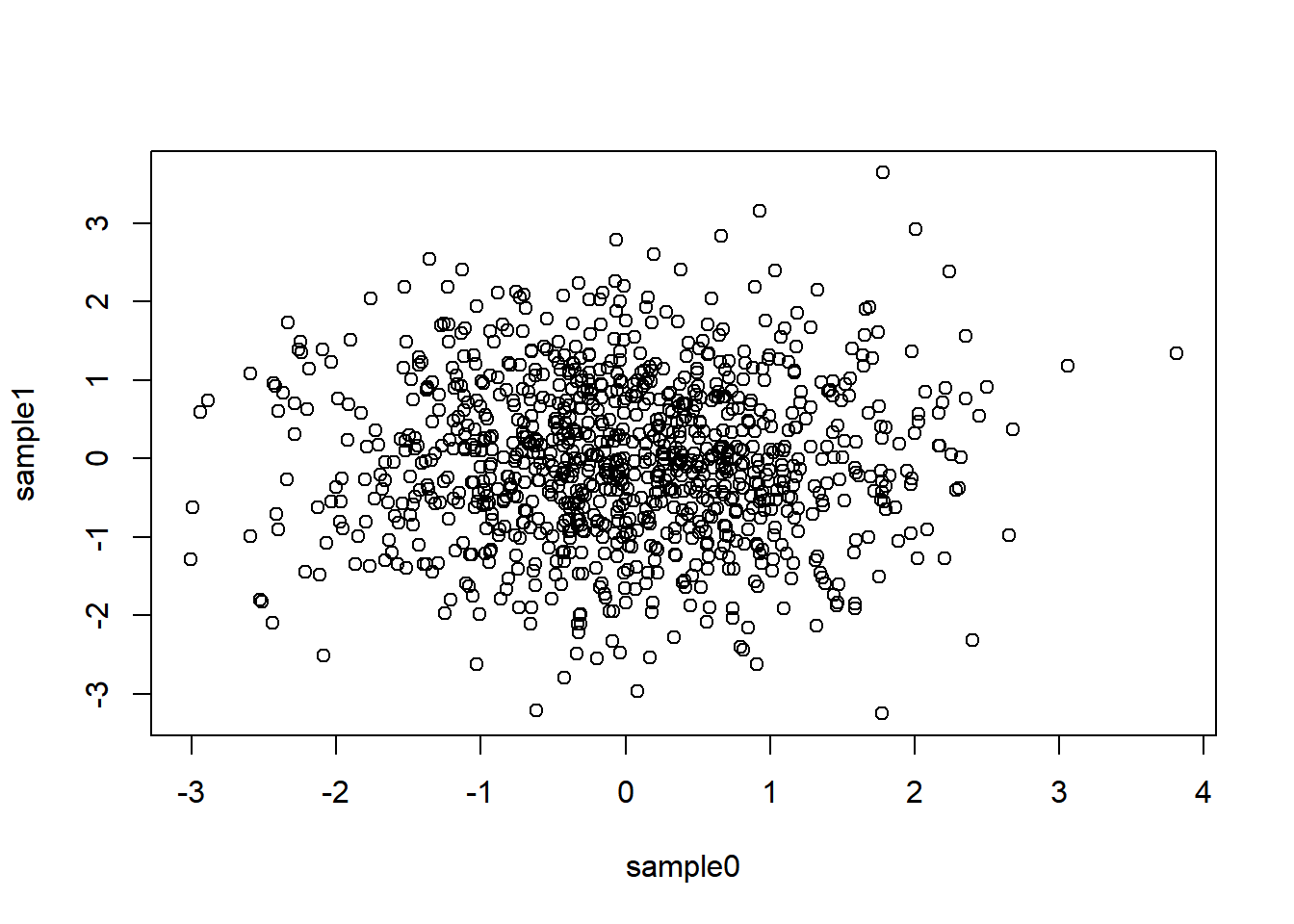
    Pearson's product-moment correlation

data:  sample0 and sample1
t = 0.20223, df = 998, p-value = 0.8398
alternative hypothesis: true correlation is not equal to 0
95 percent confidence interval:
 -0.05561394  0.06836716
sample estimates:
        cor
0.006401211
cor.test(sample0, sample1, method='spearman')
    Spearman's rank correlation rho

data:  sample0 and sample1
S = 168382440, p-value = 0.745
alternative hypothesis: true rho is not equal to 0
sample estimates:
        rho
-0.01029565
cor.test(sample0, sample1, method='kendall')
    Kendall's rank correlation tau

data:  sample0 and sample1
z = -0.32648, p-value = 0.7441
alternative hypothesis: true tau is not equal to 0
sample estimates:
         tau
-0.006894895
Warning in cor.test.default(Cars93$Weight, Cars93$Price, method = "spearman"):
Cannot compute exact p-value with ties
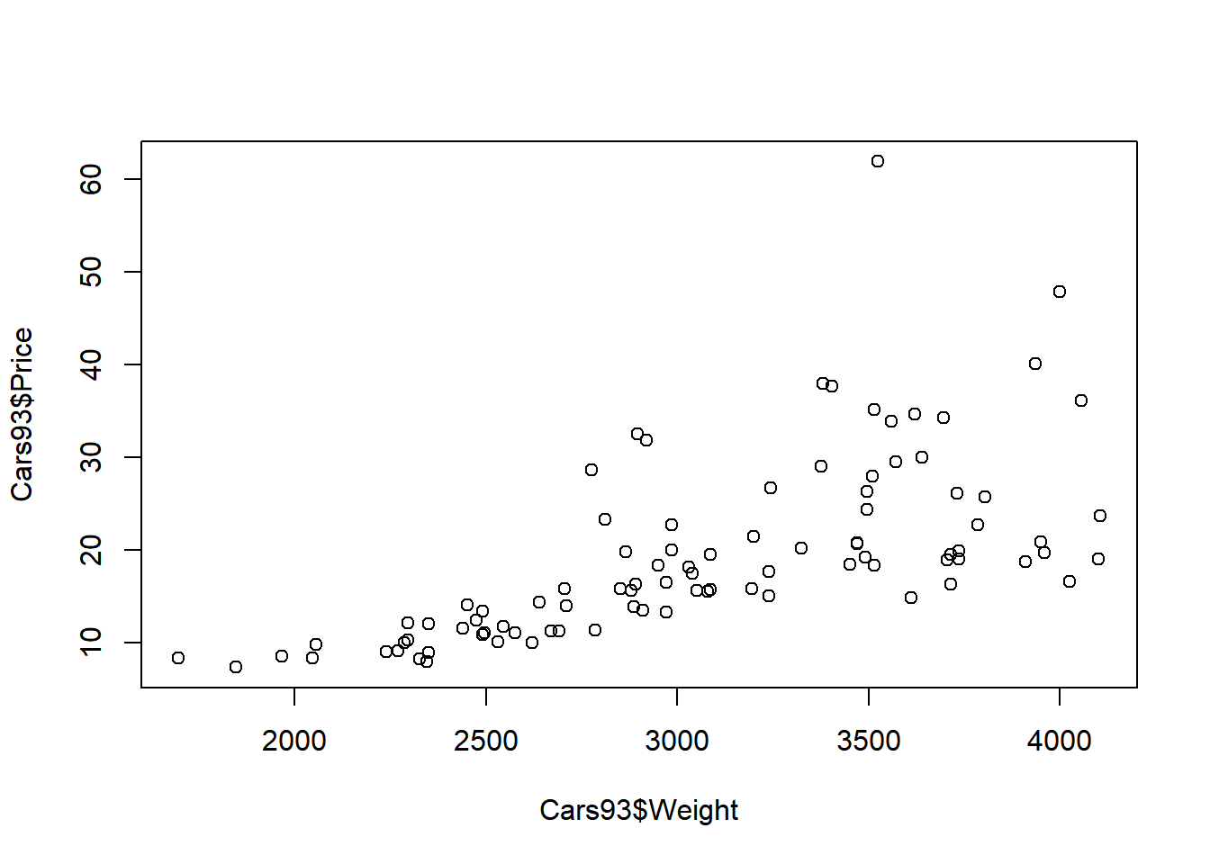
    Spearman's rank correlation rho

data:  Cars93$Weight and Cars93$Price
S = 29343, p-value < 2.2e-16
alternative hypothesis: true rho is not equal to 0
sample estimates:
      rho
0.7810954
    Kendall's rank correlation tau

data:  Cars93$Weight and Cars93$Price
z = 8.3879, p-value < 2.2e-16
alternative hypothesis: true tau is not equal to 0
sample estimates:
      tau
0.5924276